Linear Regression and Cost function

In this part of this exercise from Coursera Machine Learning, I will implement linear regression with one variable to predict profits for a food truck. Matlab is the tools I used for this project. Link to Github

Plotting the data

The first figure shows the scatter plot of profit and population in the city. Scatter plot and linear line

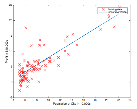
The scatter plot of the training data reveals the positive relationship between profit and population. Also, the blue line is the regression line.

function plotData(x, y)

  plot(x, y, 'rx', 'MarkerSize', 10); % Plot the data 
  ylabel('Profit in $10,000s'); % Set the y?axis label 
  xlabel('Population of City in 10,000s'); % Set the x?axis label

  figure; % open a new figure window

end

Gradient descent

In this part, I will fit the linear regression parameters θ to our dataset using gradient descent. The objective of linear regression is to minimize the cost function

J = sum((X * theta - y) .^ 2) / (2*m);

where the hypothesis h0(x) is given by the linear model

For population = 35,000, we predict a profit of 4519.767868
For population = 70,000, we predict a profit of 45342.450129

% Predict values for population sizes of 35,000 and 70,000
predict1 = [1, 3.5] *theta;
predict2 = [1, 7] * theta;

Next, the implementation of gradient descent is in gradientDescent.m

function [theta, J_history] = gradientDescent(X, y, theta, alpha, num_iters)

m = length(y); % number of training examples
J_history = zeros(num_iters, 1);

for iter = 1:num_iters
    theta = theta - (alpha/m) * (X' * (X * theta - y));
    J_history(iter) = computeCost(X, y, theta);
end

end

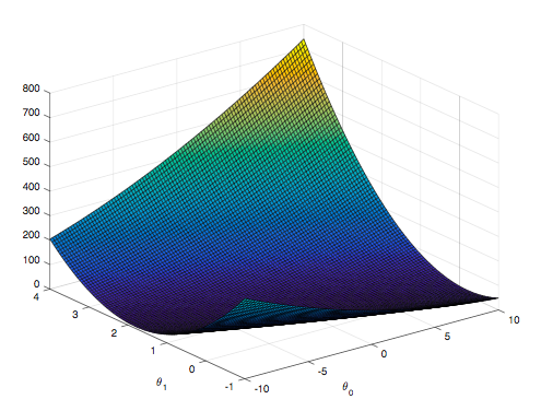
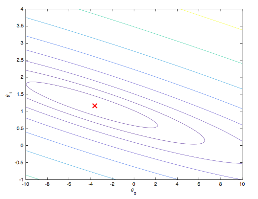
Visualizing J(theta_0, theta_1)

Surface plot

Contour plot

fprintf('Visualizing J(theta_0, theta_1) ...\n')

% Grid over which we will calculate J
theta0_vals = linspace(-10, 10, 100);
theta1_vals = linspace(-1, 4, 100);

% initialize J_vals to a matrix of 0's
J_vals = zeros(length(theta0_vals), length(theta1_vals));

% Fill out J_vals
for i = 1:length(theta0_vals)
    for j = 1:length(theta1_vals)
	  t = [theta0_vals(i); theta1_vals(j)];    
	  J_vals(i,j) = computeCost(X, y, t);
    end
end


% Because of the way meshgrids work in the surf command, we need to 
% transpose J_vals before calling surf, or else the axes will be flipped
J_vals = J_vals';
% Surface plot
figure;
surf(theta0_vals, theta1_vals, J_vals)
xlabel('\theta_0'); ylabel('\theta_1');

% Contour plot
figure;
% Plot J_vals as 15 contours spaced logarithmically between 0.01 and 100
contour(theta0_vals, theta1_vals, J_vals, logspace(-2, 3, 20))
xlabel('\theta_0'); ylabel('\theta_1');
hold on;
plot(theta(1), theta(2), 'rx', 'MarkerSize', 10, 'LineWidth', 2);

Full source code: Github

Lanbig