Ensemble Classifier - Machine Learning

Boosting and Bagging are said to be methods that can improve classification algorithm performance. Having also learned multiple ensemble classifier methods, we wonder which methods between Boosting and Bagging can be outperformed for prediction accuracy improvement. Our goals are to experiment different types of weak-learner-based ensemble classifier with boosting and bagging parameters, and compare them with the performance evaluation procedures.

The full source code is in Github Gist

Required library list.

require(caret)
require(ggplot2)
require(randomForest)
require(e1071)
require(pROC)
require("foreach")
require("doSNOW")
require(party)

Data Preprocessing

Our data set consists of 5 malignancy ratings (1, 2, 3, 4 and 5) given by 4 different radiologists, we then decide to bin the classes by grouping them into 2 classes -class 1, 2, 3 and class 4 and 5 as inconclusive and likely suspicious of malignancy respectively.

myd = read.csv("Lung Cancer dataset/LIDC_Data_SEIDEL_01-05-2015.csv",header = T, sep = ',')
mycl = data.frame(matrix(NA, ncol = 1, nrow = nrow(myd)) )
names(mycl)[1]<-paste("class")

for(i in 1:nrow(myd))
{
  row <- myd[i,]
  avg <- (row[5]+row[6]+row[7]+row[8])/4
  mycl[i,1] <-  ifelse(avg >=4 , "Likely", "Inconclusive")
}

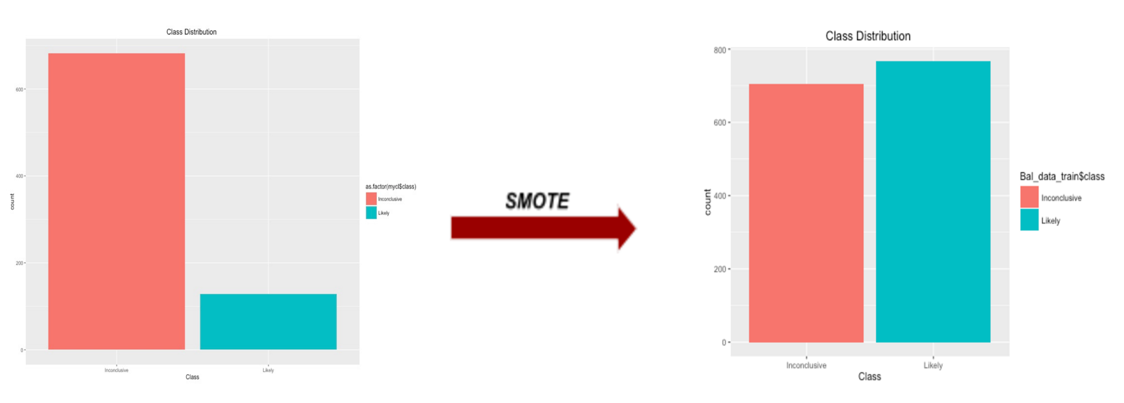
qplot(mycl$class, geom="bar",ylab = "count", main = "Class Distribution ", xlab = "Class", fill=as.factor(mycl$class)) 

we can obviously see the data become imbalanced with inconclusive and likely class, 682 and 128 respectively. Minorities would be ignored from the model prediction. We resolved this issue by applying SMOTE function in DMwR library on raw data. With this function, it is said by Torgo, L. (2010) to artificially generate new examples from the minority class using the nearest neighbors of these cases, and majority class examples are also under-sampled, leading to a more balanced dataset.

########   SMOTE   ########
######## Balance the data set, comment this part if you don't want ########
require(DMwR)
sdata = cbind(train_Y,train_X)
names(sdata)[1]<-paste("class")

Bal_data_train <- SMOTE(class ~ ., sdata, perc.over = 500,perc.under=110)
table(Bal_data_train$class)
qplot(Bal_data_train$class, geom="bar",ylab = "count", main = "Class Distribution ", xlab = "Class", fill=Bal_data_train$class ) 

train_X = Bal_data_train[,2:65]
train_Y = as.factor(Bal_data_train[,1])

Ensemble Tree

Principle Component Analysis (PCA) is the feature extraction technique that can reduce the dimension space of the data set. This data set has many attributes (more than 60 attributes). After applying PCA, the first feature we extract from the attribute space captures the most variability in the data.

#######   Feature Extraction     #######
#######    Extract new feature, reduce feture dimention, #######
#######     comment this part if you don't want #######
require(clusterSim)
fdata = cbind(train_Y,train_X)
Norm_data_train = data.Normalization(fdata[2:65],type="n4",normalization="column");

#Apply PCA
data_train.pca <- princomp(Norm_data_train, cor = TRUE, center = TRUE, scale. = TRUE) 
plot(data_train.pca)
summary(data_train.pca)

train_X = data_train.pca$scores[,1:22]
train_Y = as.factor(Bal_data_train[,1])

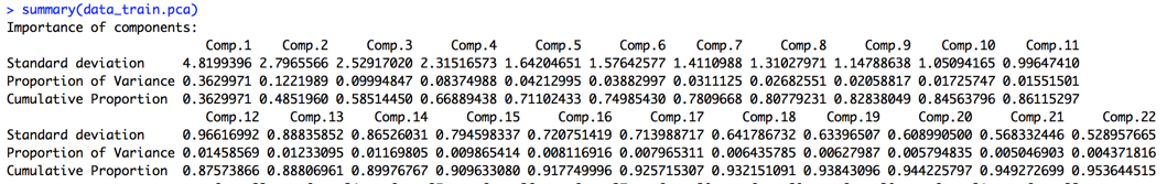Ensemble Tree we then decide to use 22 components to capture at least 95 percent of the variances in the data.

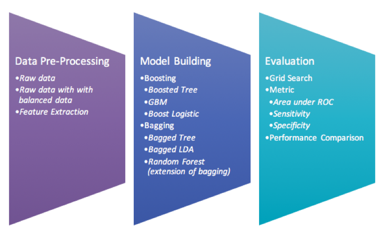
Model Fitting

Step for model building Ensemble Tree

Apply the three data set with Boosting and Bagging modeling techniques.
Perform grid search to find the best parameter for each best model.
Use 10 folds-cross validation in order to avoid model overfitting

#############################################
fitControl <- trainControl(method = "repeatedcv",
                           repeats = 10,
                           number = 10,
                           #summaryFunction = multiClassSummary,
                           summaryFunction = twoClassSummary,
                           savePredictions =T,
                           verboseIter = TRUE,
                           ## Estimate class probabilities
                           classProbs = TRUE)

#############################################

fit.rf = train(y = train_Y, x = train_X, method= "rf"  , 
                  tuneLength = 5,
                  metric="ROC",
                  trControl = fitControl)
plot(fit.rf)
fit.rf

pred <- predict(fit.rf, train_X)
xtab <- table(pred, train_Y)
confusionMatrix(fit.rf)

#############################################

fit.ada = train(y = train_Y, x = train_X, method= "ada"  , 
               metric="ROC",
               trControl = fitControl)
plot(fit.ada)
fit.ada

trellis.par.set(caretTheme())
plot(fit.ada, metric = "ROC", plotType = "level",
     scales = list(x = list(rot = 90)))

#############################################

fit.treeBag = train(y = train_Y, x = train_X, method= "treebag", 
                    metric="ROC",
                    trControl = fitControl)
plot(fit.treeBag)
fit.treeBag

#############################################
fit.LogitBoost = train(y = train_Y, x = train_X, method= "LogitBoost", 
                    metric="ROC",
                    tuneLength = 8,
                    trControl = fitControl)
plot(fit.LogitBoost)
fit.LogitBoost

#############################################

fit.AdaM1 = train(y = train_Y, x = train_X, method= "AdaBoost.M1", 
                       metric="ROC",
                       trControl = fitControl)
plot(fit.AdaM1)
fit.AdaM1

#############################################

fit.gbm = train(y = train_Y, x = train_X, method= "gbm", 
                  metric="ROC",
                  trControl = fitControl)
plot(fit.gbm)
fit.gbm

#############################################

fit.bagLDA <- train(train_X, train_Y, 
                 "bag", 
                 B = 10, 
                 trControl = fitControl,
                 bagControl = bagControl(fit = ldaBag$fit,
                                         predict = ldaBag$pred,
                                         aggregate = ldaBag$aggregate),
                 tuneGrid = data.frame(vars = c((1:10)*10 , ncol(train_X))))
plot(fit.bagLDA)
fit.bagLDA


###### Perf ######

resamps <- resamples(list(RF = fit.rf,
                          BoostedTree = fit.ada,
                          BaggedCart = fit.treeBag,
                          LogitBoost= fit.LogitBoost,
                          BaggedLDA = fit.bagLDA,
                          GBM = fit.gbm
                          ))
resamps
summary(resamps)
bwplot(resamps, layout = c(5, 1))

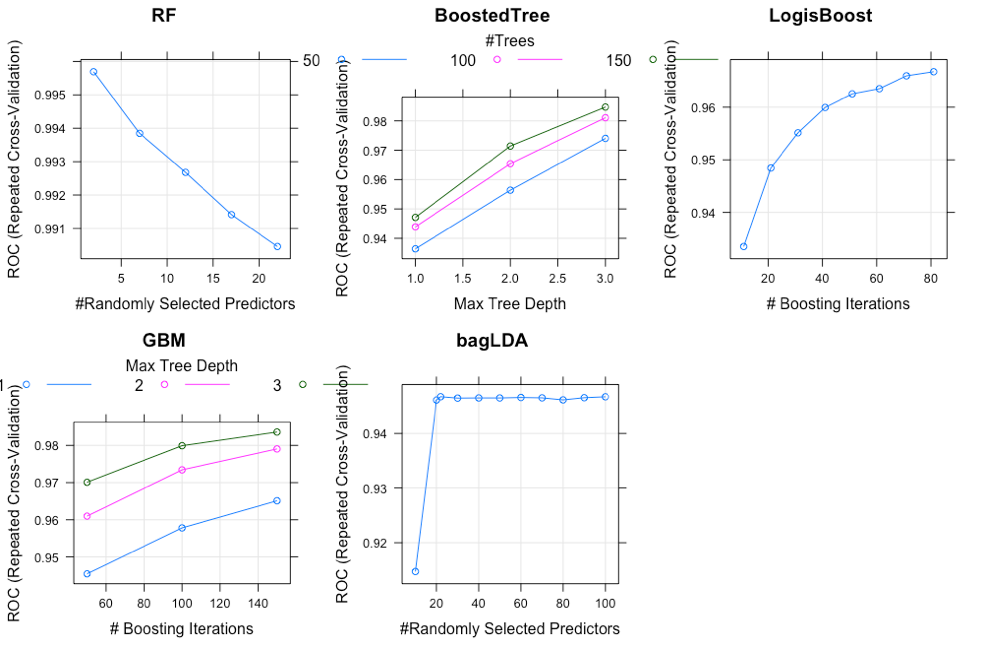
Experimental Results

Grid Search has been performed to find the best parameters for each model and this plot just shows an example of how the models performed with different parameters Ensemble Tree

Performance Evaluation

Having fitted all models on each data set, we can see the the Random Forest has the best overall performance, even though the Boosted tree perform better in only imbalanced data. The second best model so far is Bagged Cart (Bagged Tree) model on both balanced and PCA data set, and Random Forest for the unbalanced data.

Ensemble Tree

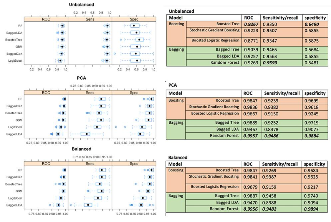
Conclusion

Based on this data set, we can conclude for these findings that Bagging is more outperformed than Boosting techniques on binary class variables, but Boosting might perform best on unbalanced data. Even though Kristína Machová found Boosting has higher performance in her work, it makes sense to us that we found Bagging has higher performance on this certain data because cross validation is used in experiment making our samples become small which fit very well in Bagging models. Within boosting technique, boosted tree perform the best across all different data. For the bagging, Random Forest perform the best among other bagging techniques (Bagged Tree and Bagged LDA).

Lanbig