Using EGARCH to forecast volatility in Microsoft Stock.
In this example, we are going to forecast the volatility of Microsoft stock. First, we will attempt to discover dataset. Our data set consists of closing prices of MSFT from January 2, 1998 to February 26, 2016. The number of observations is equal to 4,567 closing prices. Our data was retrieved from the Yahoo! Finance website under historical data. Here is plot of the time series
Let’s start with exploratory analysis of the data
library(rugarch)
library(ggplot2)
library(zoo)
library(fBasics)
library(fUnitRoots)

myd= read.table('MSFT.csv', header=T, sep=',')
myd_lim = myd[1:4567,]
pricets = zoo(myd_lim$Adj.Close, as.Date(as.character(myd_lim$Date),format=c("%Y-%m-%d")))

autoplot(pricets)
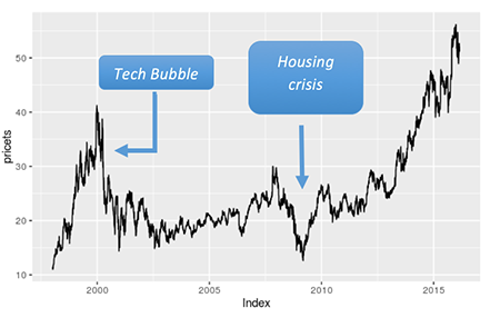
Originally, we took the data set from the IPO (Initial Public Offering) date of March 13, 1986. However, there was too much of trend since the stock has split many times. With this in mind, we decided to start to our data set in February of 1998. As you can see there is a steep run up during the dot com bubble of the late 1990’s and early 2000. The tech bubble peaked on March 10, 2000. Next there was a steep drop, and then the stock hung around 20 for years. Then during the Mortgage crisis the stock dropped down into the teens, bottoming in 2009. Since the company made Satya Nadella the CEO, the stock has had a nice rally up to the volatility of early 2016.
Next, we going to use acf for checking non-stationary behavior.
acf(coredata(pricets))
# the ACF function of the first difference
dx=diff(coredata(pricets))
acf(as.vector(dx),lag.max=30, main="ACF of first difference")
adfTest(dx, lags=3, type=c("ct"))
adfTest(dx, lags=5, type=c("ct"))
adfTest(dx, lags=7, type=c("ct"))
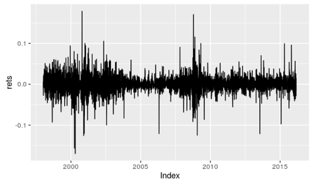
rets = log(pricets/lag(pricets, -1))
head(rets)
basicStats(rets)
autoplot(rets)
The ACF plot(below) of the squared log returns of MSFT decays very slowly. The lags are all much larger than 2 standard deviations. This confirms large autocorrelations in the squared log returns. Therefore we can conclude that the log returns process has a strong non-linear dependence.
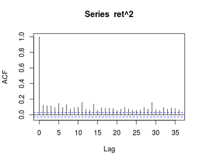
Since we have confirmed serial correlation in the conditional variance of the process, we can say that the conditional variance of the process at time t is a function of the variance at previous times. Therefore we can use the past to explain or predict the current variance. This enables us to use GARCH model to model the variance of the MSFT stock price time series.
Model Fitting
This enables us to use GARCH model to model the variance of the MSFT stock price time series. Model fitting There were 4 models applied to MSFT stock:
-
GARCH with normally distributed errors
-
GARCH with T distributed errors
-
EGARCH with T distributed errors
-
TGARCH with T distributed errors
As a result, EGARCH model turned out to be the best one based on BIC. Below was the model we selected because it was the best fit.
#MODEL 3: AR(0)-EARCH(1,1) with T distributed errors
egarch11.t.spec=ugarchspec(variance.model=list(model = "eGARCH",
                                                 garchOrder=c(1,1)), mean.model=list(armaOrder=c(0,0)),
                             distribution.model = "std")
egarch11.t.fit=ugarchfit(spec=egarch11.t.spec, data=rets)
egarch11.t.fit
plot(egarch11.t.fit)
> egarch11.t.fit

*---------------------------------*
*          GARCH Model Fit        *
*---------------------------------*

Conditional Variance Dynamics
-----------------------------------
GARCH Model	: eGARCH(1,1)
Mean Model	: ARFIMA(0,0,0)
Distribution	: std

Optimal Parameters
------------------------------------
        Estimate  Std. Error    t value Pr(>|t|)
mu      0.000163    0.000192    0.85054 0.395022
omega  -0.045584    0.002250  -20.25762 0.000000
alpha1 -0.033122    0.008084   -4.09718 0.000042
beta1   0.994380    0.000360 2762.66379 0.000000
gamma1  0.118418    0.009921   11.93615 0.000000
shape   4.960095    0.338704   14.64433 0.000000

Robust Standard Errors:
        Estimate  Std. Error    t value Pr(>|t|)
mu      0.000163    0.000202    0.80726 0.419514
omega  -0.045584    0.004711   -9.67646 0.000000
alpha1 -0.033122    0.009556   -3.46629 0.000528
beta1   0.994380    0.000559 1778.11697 0.000000
gamma1  0.118418    0.012053    9.82473 0.000000
shape   4.960095    0.379098   13.08394 0.000000

LogLikelihood : 12249.67
Now, we are going to look into the result.
-
AR(0) mean model with standard EGARCH(1,1) model for variance & t-distribution has been selected for the best model.
-
Fitted model: rt = 0.000163 + at, at=σtet and ln(σ2t) = -0.045584 + (-0.033122 et-1 + 0.118418(|et-1| - E(|et-1|)) + 0.994380 ln(σ2t-1) With t distribution with 5 degrees of freedom (approximated to nearest integer).
-
Alpha1 is negative (= -0.033). Leverage effect is significant. Therefore volatility reacts more heavily to negative shocks.
-
Beta1 represents persistence of shocks on volatility. Our 1 = .99438 which is very high. Strong, long lasting persistence. Transition smoother and takes a long time from high to low volatility.
-
We used the BIC criteria to select the best model. This model had the smallest BIC at -5.3545 of the 4 models we created.
-
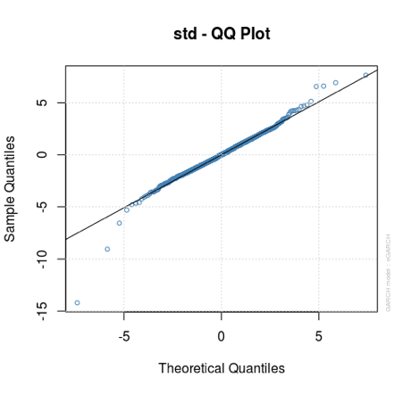
Pearson Goodness of Fit Test H0: selected distribution is a good fit for model Ha: selected distribution not a good fit The p-values > .05 . Therefore we can’t reject the hypothesis that the selected t-distribution is a good fit for the model.
T-distribution probability plot(left) for residuals show that t-distribution is appropriate. Some departure is seen under the left tail for extreme residuals (associated to extremely low returns)
Residual analysis and model diagnostics
Weighted Ljung-Box Test on Standardized Residuals
------------------------------------
                        statistic p-value
Lag[1]                      1.015  0.3136
Lag[2*(p+q)+(p+q)-1][2]     1.299  0.4107
Lag[4*(p+q)+(p+q)-1][5]     2.711  0.4623
d.o.f=0
H0 : No serial correlation

Weighted Ljung-Box Test on Standardized Squared Residuals
------------------------------------
                        statistic p-value
Lag[1]                    0.03079  0.8607
Lag[2*(p+q)+(p+q)-1][5]   0.13676  0.9965
Lag[4*(p+q)+(p+q)-1][9]   0.23303  0.9999
d.o.f=2

Weighted ARCH LM Tests
------------------------------------
            Statistic Shape Scale P-Value
ARCH Lag[3]   0.01272 0.500 2.000  0.9102
ARCH Lag[5]   0.17060 1.440 1.667  0.9723
ARCH Lag[7]   0.19333 2.315 1.543  0.9973
-
Ljung Box tests for white noise behavior in residuals show that there is no evidence of autocorrelation in residuals. They behave as a white noise process.
-
Tests for ARCH/GARCH behavior in residuals reveal that there evidence of serial correlation in squared residuals. They behave as a white noise process.
After conducting tests on the residuals, we can conclude the residuals behave as white noise and are random. Therefore our model has captured the behavior of the volatility.
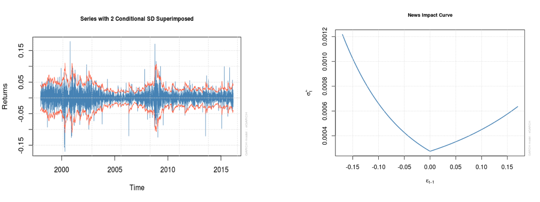
The plot on the left below shows the volatility of the MSFT stock return with 2 Conditional SD. Most of the time, the EGARCH model performed very well in order to capture the negative outliers or negative shocks. However, the model might not be able to capture the extreme shocks or outliers.
The News Impact Curve(below right) reiterates the fact that in our model the leverage effect is significant and that the volatility of our data set reacts more strongly to negative shocks than to positive shocks. You can see by looking at the graph that the magnitude of the volatility skyrockets as the shocks are more negative.
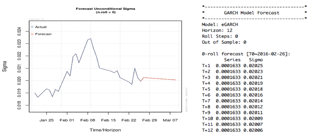
Forecast analysis
Based on the analysis, EGARCH(1,1) model for variance and t-distribution turned out to be the best model BIC supports using the EGARCH model better than the GARCH model and TGARCH model. Forecasts are computed using the ugarchforecast function for the next 12-step ahead. The plot of the forecast unconditional sigma shows that the stock volatility will slightly decrease in the next 12-step ahead.
Sum up
After running ACF tests and Dickey Fuller tests on the time series and first difference of the time series, we conclude the MSFT stock returns are non-stationary. Our ACF tests on log returns squared along with our failure to reject the null hypothesis of the Box-Ljung Test on the residuals leads us to conclude there is an ARCH Effect. After finding the ARCH Effect we used 4 different GARCH Models to model the volatility. Using the BIC Criteria, Pearson Goodness of Fit, and Residual analysis that our AR(0) EGARCH(1,1) with t-distribution is an adequate fit as a model for the data.
The best model we found showed that MSFT stock reacts more violently to negative news than it does positive news. When bad news comes out like bad earnings, terrorism, or poor economic data, MSFT price tends to go down faster and farther than when good news comes out and the stock rises. Also, the transition from periods of rapid price changes to periods of stable prices is fairly smooth and takes longer in MSFT compared to some other securities.