Lanbig

Online News Popularity data set has been selected from the UC Irvine Machine Learning Repository Link. The articles in this data set were published by Mashable. This data set is donated on January 8, 2015. The data set includes 39797 observations and 61 combined attributes. The goal of this project is to find non-trivial, potential useful knowledge and predict the popularity of the articles, which is the number of shares in social networks.

• The explanatory attributes for Online News Popularity data set include URL of the article, number of words in the title, number of words in the content, number of images, number of videos, polarity of positive words and polarity of negative words are numeric. These attributes can be used to create a predictive model.
• The response attribute is the number of shares in social network (popularity).

The full source code is in Github Gist

###########Required Library##########
library(rpart.plot)
library(caret)
library(e1071)
library(klaR)
library(rattle)
library(rpart.plot)
library(RColorBrewer)
library(ggplot2)

Data Exploratory

library(ggplot2)
theme_set(theme_bw(base_size = 28))

qplot(df.onNews$dataChannel, geom="histogram",ylab = "count",binwidth = 30,
      main = "Histogram for data channel", xlab = "Channel", fill=df.onNews$share2bins ) 

qplot(df.onNews$pubDay, geom="histogram",ylab = "count",binwidth = 30,
      main = "Histogram for publication day", xlab = "Day", fill=df.onNews$share2bins ) 

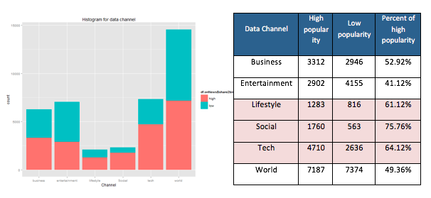
Most positive cases (high popularity) are captured in Lifestyle, social and tech channel. These channels seem to be much popular than business, entertainment and word channel. For example, Social channel had 76 percent of positive cases (high popularity) and technology channel had 64 percent of positive cases.

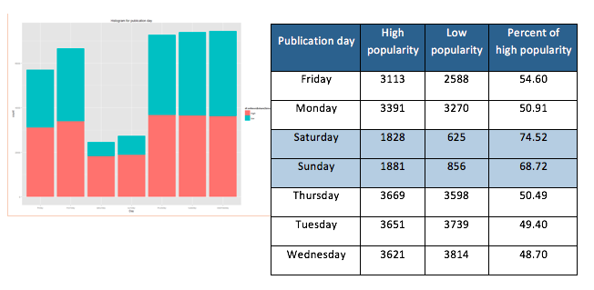
In reviewing positive cases (high popularity) on the publication day, most news shared on weekend seems to be in the “high popularity” group. About 75 percent of the news published on Sunday was popular. The news published on weekday tent to be in “low popularity” group. For example, the majority of the news shared on Wednesday and Tuesday were unpopular.

Model Fitting

In this data set, we’ll define an 66%/34% for training and test data.

set.seed(415)
# define an 66%/34% train/test split of the dataset
trainIndex <- createDataPartition(df.onNews$share2bins, p=0.66, list=FALSE)
data_train <- df.onNews[ trainIndex,]
data_test <- df.onNews[-trainIndex,]

Decision Tree Analysis

fit.rpart8= train(share2bins ~ . ,data=data_train , method= "rpart", tuneLength = 8, trControl=trainControl(method="cv",number=10))

> print(fit.rpart8)
CART 

26166 samples
   47 predictor
    2 classes: 'high', 'low' 

No pre-processing
Resampling: Cross-Validated (10 fold) 
Summary of sample sizes: 23550, 23550, 23548, 23550, 23549, 23550, ... 
Resampling results across tuning parameters:

  cp           Accuracy   Kappa       Accuracy SD  Kappa SD  
  0.003605375  0.6339914  0.25555564  0.009806259  0.02197829
  0.004629630  0.6331886  0.25559910  0.007883932  0.01681616
  0.008030154  0.6297105  0.25140243  0.006750814  0.01460905
  0.008767617  0.6284876  0.24931886  0.006772829  0.01474812
  0.014175680  0.6216475  0.23057982  0.009779804  0.01893964
  0.020567027  0.6144631  0.21667075  0.011735050  0.02443565
  0.040560472  0.6005906  0.19493916  0.012689902  0.02248112
  0.124713209  0.5495640  0.05205161  0.025837704  0.08415047

Accuracy was used to select the optimal model using  the largest value.
The final value used for the model was cp = 0.003605375.

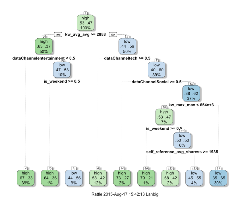
fancyRpartPlot(fit.rpart8$finalModel)

The visualization below shows the tree structure and the branches of tree. The most important five OnlineNewsPopularity data features are kw_avg_avg, data channel entertainment, data channel tech, is_weekend and dataChanelSocial. These features are on the top of the decision tree and they have the most important power to separate the classes.

Naïve Bayes Analysis

This technique is based applying Bayes’ theorem. One significant benefit of using Naïve Bayes Analysis is that it can be very fast compared to Random Forest modeling technique or other methods.

> fit.nb= train(share2bins ~ . ,data=data_train , method= "nb", trControl=trainControl(method="cv",number=10))

> fit.nb
Naive Bayes 

26166 samples
   47 predictor
    2 classes: 'high', 'low' 

No pre-processing
Resampling: Cross-Validated (10 fold) 
Summary of sample sizes: 23549, 23550, 23550, 23550, 23549, 23549, ... 
Resampling results across tuning parameters:

  usekernel  Accuracy   Kappa       Accuracy SD  Kappa SD  
  FALSE      0.5198759  0.08688965  0.03318579   0.05532158
   TRUE      0.5998991  0.21353378  0.02759259   0.04304326

Random Forest Analysis

From the Kaggle competitions, random forest analysis tends to do very well and scoring high on the Kaggle leaderboard because a random forest analysis improves predictive accuracy by generating a large number of bootstrapped trees (boosting mechanisms)

> fit.rf = train(share2bins ~ . ,data_train , method= "rf", ntree=501 , tuneGrid = data.frame(mtry = 4), 
+                allowParallel=TRUE,trControl=trainControl(method="cv",number=10) )
> 
 
Random Forest 

26166 samples
   47 predictors
    2 classes: 'high', 'low' 

No pre-processing
Resampling: Cross-Validated (3 fold) 
Summary of sample sizes: 17444, 17444, 17444 
Resampling results

  Accuracy   Kappa      Accuracy SD  Kappa SD  
  0.6651762  0.3222725  0.006759968  0.01355711

Tuning parameter 'mtry' was held constant at a value of 4

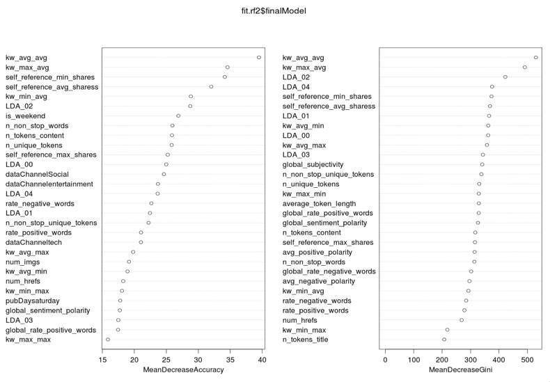
The visualization below reveals the important variables used in splitting nodes down the tree. For example, the most important Online News Popularity dataset features are Is_weekend, Kw_avg_avg, Datachanel and Self_reference variables. Most important features from a random forest analysis are about the same with decision tree analysis.

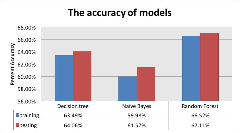
Performance Evaluation

As a result, Naïve Bayes does not work very well with the dataset. Decision tree is one the useful modeling technique since this technique is easy to interpret and understand the result. Moreover, random forest analysis is the best modeling technique with the dataset because it gets the highest accuracy in both training and testing dataset.

For recommendation and future action, there are some outliers in the variables and these outliers may impact on the accuracy of the predictive models.